There’s a mistake we see every month in camera test labs around the world: a team buys an 80:1 reflective OECF chart to characterize a brand-new HDR sensor that claims 14 stops of dynamic range. They run the test, get a measurement of about 6.5 stops, and conclude that “the sensor doesn’t perform as advertised.”
The sensor performs exactly as advertised. The test was wrong.
This guide will walk you through how to actually measure a camera’s dynamic range — properly, repeatably, and in a way that produces results you can defend in front of customers, certification bodies, and your engineering team. We’ll cover what OECF actually is, the three different definitions of “dynamic range” you’ll encounter in industry literature, the precise step-by-step procedure per ISO 15739:2023, when to use transmissive vs reflective charts (the most common decision error), how to interpret the numbers, and the four mistakes that consistently produce wrong results.
By the end, you’ll be able to set up a complete dynamic range characterization workflow from scratch, and explain to anyone in your organization exactly what your numbers mean.
Let’s start with the most fundamental concept: OECF.
What Is OECF (and Why It Matters for Dynamic Range)
OECF stands for Opto-Electronic Conversion Function. It is the mathematical relationship between scene luminance (the light hitting the camera) and the digital values the camera outputs.
Mathematically, OECF is simply: DV = f(L), where DV is the digital value (e.g., 0-255 for 8-bit) and L is the scene luminance. If you plot DV on the vertical axis and log(L) on the horizontal axis, you get the OECF curve — a graph that shows exactly how the camera maps light to numbers.
This curve is the foundation for almost every objective image quality measurement. From the OECF curve, you can derive:
- Dynamic range — from the highest unclipped luminance to the lowest detectable luminance
- Signal-to-noise ratio (SNR) — at any specific luminance level
- ISO sensitivity (ISO speed) — per ISO 12232:2019
- Gamma / tonal response curve — the slope of the OECF
- White balance accuracy — by comparing R, G, B OECF curves
- Tone mapping behavior (the “shoulder” near highlights, the “toe” near shadows)
For dynamic range specifically, the OECF curve tells you two critical things at the same time: where the sensor saturates (the highest measurable luminance) and where the noise overwhelms the signal (the lowest measurable luminance). The ratio between those two points is the dynamic range.
You cannot measure dynamic range without first measuring OECF. They’re the same measurement.
The Three Definitions of “Dynamic Range”
Before going into procedure, we need to clarify a definition problem that causes endless confusion in industry literature.
When a camera marketing document says “this sensor has 14 stops of dynamic range,” it can mean any of three different things — and they produce wildly different numbers for the same sensor.
Definition 1: Engineering Dynamic Range (EDR)
The ratio of the maximum unclipped signal to the signal level where SNR = 1.
Mathematically:
DR (stops) = log₂ (L_saturation / L_SNR=1)
Where L_saturation is the scene luminance that just barely fills the pixel wells without clipping, and L_SNR=1 is the luminance where the temporal SNR drops to 1 (0 dB) — the level where signal and noise are equal magnitude.
This is the most permissive definition. SNR=1 means the noise is as large as the signal — visually, this is extremely noisy data that most photographers and ADAS engineers would consider unusable. But sensor engineers like this definition because it represents the theoretical capability of the sensor without quality judgment.
EDR is what most sensor data sheets report. A typical full-frame DSC at base ISO might report 14 stops of EDR.
Definition 2: Photographic (or Usable) Dynamic Range (PDR)
The ratio of maximum signal to the signal level where SNR reaches a “usable” threshold — typically SNR = 10 (20 dB), but sometimes SNR = 5 (~14 dB) or SNR = 20 (~26 dB) depending on the source.
PDR (stops) = log₂ (L_saturation / L_SNR=threshold)
This is the stricter definition. A higher SNR threshold means cleaner shadow detail and a smaller reported dynamic range. ARRI, for example, measures its cinema cameras to a stringent SNR threshold, which is why ARRI’s “14+ stops” figure holds up in real-world cinematography — it represents genuinely usable stops, not theoretical capability.
The same sensor might report 14 stops EDR and only 8-9 stops PDR. Both numbers are correct; they answer different questions.
Definition 3: Scene-Referred Dynamic Range (ISO 15739:2023 §6.3)
The ratio of the input signal saturation level to the minimum input signal level that can be captured with a signal-to-temporal noise ratio of at least 1.
This is the official ISO definition. It is identical to EDR in mathematical form, but the standard adds specific requirements: the SNR must be computed from temporal noise (multi-frame averaging to separate temporal from fixed-pattern noise), the OECF must be measured per ISO 14524, and the camera must operate in its specified working range.
When CalibVision, Imatest, Image Engineering, or any ISO-compliant test lab reports “dynamic range per ISO 15739:2023,” this is the definition being used. It’s the only definition that’s standardized internationally.
Which One to Use
For most engineering and quality-assurance contexts, report the ISO 15739:2023 definition (Definition 3) as the primary number, then optionally include the photographic DR (Definition 2) at SNR=10 or SNR=20 as a complementary “usable stops” metric for downstream stakeholders.
If you only report one number, make it the ISO 15739 number, and clearly label it. The vast majority of confusion in cross-team and cross-vendor DR discussions comes from people comparing engineering DR from one source to photographic DR from another and concluding “the numbers don’t match” — when in fact they do, just measured differently.
For the rest of this guide, “dynamic range” means ISO 15739:2023 dynamic range unless explicitly stated otherwise.
Equipment Checklist
A complete OECF / dynamic range measurement workflow needs five pieces of equipment.
- OECF Test Chart
The chart provides a known set of luminance levels (via different patch densities) that the camera captures simultaneously. The choice between transmissive and reflective is critical — we’ll cover this in detail in the next section.
For ISO 15739:2023 measurements, the chart should conform to ISO 14524 OECF specifications. There are three common patch arrangements:
- 20-patch ellipse (ISO 14524 standard) — densities 0.05 to 2.85
- 15-patch simplified (Imatest popular variant) — 12 peripheral + 3 central, densities 0.1 to 2.0
- 36-patch log-uniform (Image Engineering TE269 style) — densities 0.05 to ~3.3 in even log spacing
The 20-patch ellipse is the most directly compliant with ISO 14524. The 15-patch simplified is the most widely used with Imatest software. The 36-patch is preferred for very high dynamic range sensors (>14 stops) where finer density steps reduce extrapolation error.
- Light Source
For transmissive (film) charts, you need a backlit lightbox with:
- D65 (or D50) illuminant — color temperature within ±200K of the target
- Spatial uniformity ≥98% across the chart area
- No measurable flicker (DC-driven or properly filtered AC)
- Sufficient brightness to drive the lightest patch (D=0.05) to camera saturation
For reflective (paper) charts, you need:
- D65 or D50 illuminants
- 45° front lighting from at least two sides (typically four sides for large charts)
- Baffles to prevent specular glare reaching the camera
- Uniform illumination across the chart (±5% typical, ±2% for premium labs)
- Camera Under Test
Whatever you’re characterizing — a smartphone, DSLR, machine vision camera, automotive ADAS camera, or sensor module on a test board. Standard requirements:
- Tripod or fixture mounting — zero vibration during capture
- Remote shutter / cable release — no shutter button vibration
- Manual exposure control — no auto-exposure during the capture
- RAW format if available — the further down the pipeline (JPEG, video), the more “cooked” the image and the less accurate the DR measurement
- Capture / Analysis Software
Several options exist:
- Imatest (Stepchart, Multicharts, Multitest modules) — the industry standard for most labs
- iQ-Analyzer (Image Engineering) — preferred for ISO 15739:2023-precise workflows
- ISO/TC 42 reference MATLAB code — free, official reference implementation
- In-house Python / C++ implementations — used by major camera manufacturers
For 90% of labs, Imatest is the right choice.
- (Optional) Densitometer
If you’re a high-rigor lab, a densitometer lets you spot-check the patch densities on a new chart against the manufacturer specification, and re-verify them periodically to track chart drift. Most production labs skip this; their chart vendor provides a calibration report instead.
The Most Important Decision: Transmissive or Reflective?
This is where the mistake in the opening anecdote happened. The team chose a reflective chart for an HDR sensor, and the chart’s physical limit capped the measurable dynamic range below the sensor’s actual capability.
Here’s the rule, derived from physics:
| Chart Type | Maximum Density (D_max) | Maximum Measurable DR | Best For |
| Reflective (matte photographic paper) | ~1.95-2.0 | ~6.5 stops | Production QC of mobile / consumer / mid-range sensors |
| Reflective (semi-gloss paper) | ~2.0-2.1 | ~6.8 stops | Same use cases as matte, slightly extended |
| Transmissive (film, low-contrast) | ~2.85 | ~9.5 stops | Most camera testing, general lab use |
| Transmissive (film, high-contrast 10,000:1) | ~3.0-4.0 | ~13-14 stops | HDR sensors, full-frame, medium-format, cinema |
| Transmissive (film, ultra-high-contrast 100,000:1) | ~4.5-5.0 | ~15-16 stops | Research-grade scientific sensors |
The density-to-stops conversion comes from a simple piece of math: every 0.3 in density corresponds to 1 f-stop, because density is log₁₀ (and 10^0.3 = 2). So D_max = 2.0 means a contrast ratio of 100:1, or log₂(100) ≈ 6.64 stops.
The Physics: Why Reflective Charts Are Capped
A reflective paper chart can never have a density above about 2.0 in practice. This is because:
- The chart is illuminated by ambient light that strikes the paper, gets absorbed or reflected, and bounces back into the camera.
- Even the darkest “black” patch reflects some small amount of light — from the surface, from inks that aren’t perfectly absorbing, from sub-surface scatter.
- Stray light from the lab environment also reaches the chart, raising the effective brightness of the darkest patches.
Together, these limit reflective charts to about 6.5 stops of measurable density range. There is no way to push past this with paper-and-ink technology.
Transmissive (film) charts solve this by:
- The chart is backlit from behind, so the “black” patches truly block almost all light.
- Film can be manufactured with optical densities up to 4-5 (depending on emulsion type).
- The chart is housed in a controlled lightbox with internal baffles that prevent stray ambient light from reaching the camera side.
A modern transmissive chart at 10,000:1 contrast (the CalibVision CV-NT-FT-20P series is one example) gives you 13.3 stops of measurable density. A 100,000:1 specialty chart gives you 16.6 stops. Plenty of headroom for almost any current sensor.
The Decision Tree
Q: What is the expected dynamic range of your sensor?
│
├── < 7 stops (older CCD, basic security cameras, embedded vision)
│        → Reflective chart is fine. 80:1 contrast paper is sufficient.
│
├── 7-10 stops (typical smartphone, machine vision, ADAS, consumer mirrorless)
│        → Reflective is borderline. Transmissive 10,000:1 is safer.
│
├── 10-14 stops (modern full-frame, cinema, premium ADAS)
│        → Transmissive 10,000:1 is required. Reflective will under-report.
│
└── > 14 stops (high-end cinema, scientific sensors, HDR pipelines)
        → Transmissive ≥ 30,000:1 strongly recommended. Or use multi-exposure techniques.
The single biggest cost-saving in a real test lab is buying a transmissive chart upfront. Yes, it’s more expensive than reflective. Yes, you also need a lightbox. But if you’re testing anything more capable than a basic security camera, the reflective chart will cap your measurement below the sensor’s actual capability, and you’ll have to upgrade anyway.
The Step-by-Step Procedure
This is the canonical procedure for ISO 15739:2023-compliant dynamic range measurement using an OECF chart.
Step 1: Mount the Chart
Place the chart flat and perpendicular to the optical axis of the camera. Any tilt introduces uneven illumination across the patches.
For transmissive charts, install in a D65 backlit lightbox. Confirm the backlight is producing uniform illumination — measure with a luminance meter at the center and at the four corners; the variation should be ≤2%.
For reflective charts, mount on a rigid backing (foam board or aluminum honeycomb) so the chart cannot warp. Install at the chart’s intended viewing angle (typically 0° — directly facing the camera).
Step 2: Set Up the Lighting
For transmissive: confirm the backlight is at D65, full intensity, and stable. Allow 15-30 minutes warmup so the light source temperature stabilizes.
For reflective: position two 45° illuminators on either side of the camera-chart axis. Confirm both illuminators are matched D65, equal output, and equal distance to the chart. Add baffles between the illuminators and the camera to prevent any direct light from reaching the lens.
Measure the illumination uniformity at the chart center and corners. The ratio between center and corner should be within ±5% (±2% for ISO 17025 labs).
Step 3: Position the Camera
Mount the camera on a tripod or fixture, perpendicular to the chart. Frame the shot so:
- The chart fills 60-80% of the central field of view (avoid the corner regions where lens vignetting is strongest).
- Each patch occupies at least 64×64 pixels in the captured image (this is the ISO 15739:2023 minimum for noise measurement).
- There is a clear margin around the chart so no chart edges reach the image boundary.
For a typical 24 MP camera at standard working distance, an M-size chart (430×640 mm) fills the frame with patches of about 150×150 pixels — plenty of headroom.
Step 4: Configure the Camera
Set the camera to:
- Manual mode — no auto-exposure between captures
- Base ISO (ISO 100 for most cameras, ISO 64 or 80 for some Sony / Nikon)
- D65 white balance (or auto if testing JPEG output specifically)
- Lowest compression — RAW format strongly preferred; if JPEG, lowest compression and minimum sharpening
- Single-shot drive mode — no burst
- Remote shutter or self-timer — eliminate vibration from shutter button press
If you’re testing JPEG output, also disable any “auto-enhancement” features like Active D-Lighting, DRO, HDR mode, or noise reduction. These all distort the OECF curve.
Step 5: Adjust Exposure to “Just Clipped”
Per ISO 15739:2023 §5.4: “The light source and diffuser shall be adjusted to give the maximum unclipped level from the camera.”
In practice:
- Take a test shot.
- Examine the histogram of the lightest patch (D=0.05).
- If the patch is below saturation, increase exposure (longer shutter or wider aperture) by one stop and re-shoot.
- If the patch is saturated (clipped), decrease exposure by 1/3 stop and re-shoot.
- Iterate until the lightest patch reads at “just clipped” — the smallest exposure step above which clipping begins.
This is the reference exposure. All subsequent captures use this exposure setting.
Step 6: Capture Multi-Frame Sets
Per ISO 15739:2023, you must capture at least 8 frames at the reference exposure, with no movement of the camera or chart between frames. The multi-frame set lets the analysis software separate temporal noise (frame-to-frame variation) from fixed-pattern noise (deterministic spatial structure).
For better statistics, capture 16-32 frames. For very low-noise sensors, more frames help the analysis stabilize. Disk space is cheap; reshoot is expensive.
Save all frames as RAW. If your camera doesn’t support RAW, save as the highest-quality JPEG available, but note in your test report that the results are JPEG-derived (these will under-report the sensor’s true DR by 1-2 stops due to the JPEG tone mapping).
Step 7: (Optional) Slightly Defocus
ISO 15739:2023 permits slight defocus to ensure the chart’s structural features don’t introduce sharpness-related artifacts into the noise calculation. The standard requires that the chart’s pattern frequency content be at least 10× lower than the camera’s limiting resolution.
In practice, perfect focus is fine for most cameras. If you have a very high-resolution camera (≥50 MP) and your chart has fine printed text or borders, defocusing by 1-2 pixels prevents the text from contaminating the patch noise statistics.
Step 8: Load Images into Analysis Software
Open Imatest Stepchart, Multicharts, or your equivalent software. Load all 8-32 captured frames. Configure:
- Chart type (Imatest dropdowns include ISO 14524, ISO 15739 simplified 15-patch, ISO 15739 20-patch, etc.)
- Patch density values (the software ships with standard density tables, or you can enter custom values from your chart’s calibration report)
- Color space and gamma (sRGB / Adobe RGB / Linear, gamma 2.2 / 1.0)
Step 9: Compute OECF and Dynamic Range
Run the analysis. The software will:
- Detect the patch locations within the image.
- Compute mean pixel value for each patch (the signal).
- Compute standard deviation across the multi-frame set for each patch (temporal noise).
- Apply Annex C low-frequency variation removal (normative in ISO 15739:2023).
- Build the OECF curve: log(L) on x-axis, DV on y-axis.
- Build the SNR curve: log(L) on x-axis, SNR (dB or linear) on y-axis.
- Identify the saturation point (highest unclipped luminance).
- Identify the SNR=1 point (where the SNR curve crosses 0 dB).
- Compute DR (stops) = log₂(L_saturation / L_SNR=1).
For high-quality DR reporting, also compute DR at SNR=10 (20 dB) as the “photographic” or “usable” dynamic range.
Step 10: Validate Results
Sanity-check your numbers against expectations:
- Smartphone main camera (2024-2026): 10-12 stops engineering DR, 6-8 stops photographic DR
- APS-C / full-frame consumer: 12-14 stops engineering, 8-10 photographic
- Premium cinema (ARRI Alexa, RED Komodo): 14-17 stops engineering, 12-14 photographic
- Automotive ADAS (typical): 14-18 stops (HDR-specific designs, multiple exposure modes)
- Older CCD security camera: 6-8 stops engineering
If your measurement is dramatically different (say, 5 stops when you expected 12), the problem is almost certainly in your setup — not the sensor. Common causes are covered next.
Worked Example with Real Numbers
Let’s work through a real example so the procedure becomes concrete. We’ll measure a hypothetical mirrorless camera at base ISO 100 with a 20-patch transmissive chart at 10,000:1 contrast.
Captured Data (after running through Imatest)
| Patch | Density | log₁₀(L) | Mean DV (16-bit raw) | σ_temporal | SNR (linear) | SNR (dB) |
| 1 | 0.05 | 4.05 | 65,520 | (saturated) | — | — |
| 2 | 0.15 | 3.95 | 56,810 | 31 | 1,832 | 65.3 |
| 3 | 0.3 | 3.8 | 40,200 | 28 | 1,436 | 63.1 |
| 5 | 0.6 | 3.5 | 20,100 | 22 | 913 | 59.2 |
| 8 | 1.05 | 3.05 | 7,150 | 14 | 511 | 54.2 |
| 11 | 1.5 | 2.6 | 2,540 | 8.5 | 299 | 49.5 |
| 14 | 1.95 | 2.15 | 902 | 5.2 | 173 | 44.8 |
| 17 | 2.4 | 1.7 | 320 | 3.8 | 84 | 38.5 |
| 18 | 2.55 | 1.55 | 227 | 3.5 | 65 | 36.2 |
| 19 | 2.7 | 1.4 | 161 | 3.3 | 49 | 33.8 |
| 20 | 2.85 | 1.25 | 114 | 3.2 | 36 | 31.1 |
Determining the Saturation Point
Patch 1 is saturated. Patch 2 (D=0.15) is the last unclipped patch. The saturation point is between D=0.05 and D=0.15 — by interpolation, the camera saturates at approximately D=0.10 (the “just clipped” point).
In linear units, this corresponds to:
L_saturation = 10^(4.05 – 0.05) = 10^4.0 = 10,000 (relative scene luminance)
Extrapolating to SNR=1
The captured patches show SNR decreasing logarithmically. By Patch 20 (D=2.85), SNR is still 36 — far above 1. We can extrapolate to find where SNR will equal 1.
Plotting log(SNR) vs density: the slope is approximately -3.5 stops/density for this sensor. From SNR=36 at D=2.85, we need to extrapolate to SNR=1, which requires an additional log₂(36) = 5.17 stops of density beyond patch 20.
5.17 stops × 0.301 (the density-per-stop) = 1.56 density units. So SNR=1 occurs at approximately D=2.85 + 1.56 = D=4.41.
This is outside the range of our chart. The 10,000:1 chart only goes to D=4.0 (saturation contrast). The extrapolation is reliable as long as the SNR curve continues linearly in log-log space, which is the case for almost all CMOS sensors.
Computing Dynamic Range
DR (stops) = log₂ (L_saturation / L_SNR=1) = (D_SNR=1 – D_saturation) / 0.301 = (4.41 – 0.10) / 0.301 = 14.3 stops engineering DR
For photographic DR at SNR=10 (20 dB):
DR (stops) at SNR=10 = (D_SNR=10 – D_saturation) / 0.301
From the data, SNR=10 occurs near patch 22 (extrapolated D ≈ 3.15).
DR at SNR=10 = (3.15 – 0.10) / 0.301 ≈ 10.1 stops photographic DR
Final Report
For this camera:
- ISO 15739:2023 dynamic range (engineering, SNR=1): 14.3 stops
- Photographic dynamic range (SNR=10): 10.1 stops
- OECF curve linear (gamma ≈ 1.0 in raw), confirming the sensor is in its linear regime
- Temporal noise σ at base ISO ≈ 3.2 DV (at the darkest measurable patch)
A typical premium mirrorless. The engineering number (14.3 stops) is what the marketing department wants. The photographic number (10.1 stops) is what the cinematographer cares about.
Four Common Errors and How to Avoid Them
These are the errors we see consistently in real test labs. Each one produces wrong numbers without producing any obvious “error message” — the test simply returns a misleading result.
Error 1: Using a Reflective Chart for HDR Sensors
Covered extensively above. Reflective charts cap measurable DR at about 6.5 stops. If your sensor’s actual DR is 12-14 stops, you’ll measure 6.5 and conclude the sensor is broken.
Fix: For any sensor with claimed DR > 7 stops, use a transmissive chart at 10,000:1 contrast or higher.
Error 2: Insufficient Frame Averaging
ISO 15739:2023 requires at least 8 frames for the temporal/fixed-pattern noise separation. Many labs shortcut this and use a single frame — which makes the noise measurement uncertain by 1.5-2 stops.
Fix: Always capture at least 8 frames. For premium sensors with very low noise, capture 32 frames. The extra capture time (a few minutes per camera) prevents weeks of debugging downstream.
Error 3: Skipping Annex C Low-Frequency Variation Removal
In ISO 15739:2017, LF variation removal (Annex C) was informative — optional. In ISO 15739:2023, it’s normative — required. Many labs running 2017-era software skip this step.
The consequence: lens vignetting and illumination shading get counted as “noise,” which falsely lowers the apparent SNR and shrinks the measured DR by 0.5-1 stop.
Fix: Confirm your analysis software is applying Annex C LF removal. In Imatest, this is built-in to the Stepchart and Multicharts modules but you should verify the option is enabled.
Error 4: Auto-Exposure or Auto-Enhancement Features Enabled
Cameras with Active D-Lighting (Nikon), DRO (Sony), Auto Lighting Optimizer (Canon), or similar features apply tone curve modifications that distort the OECF. The resulting “OECF” is not the sensor’s response — it’s the response with one or more processing steps applied.
This makes the measurement non-portable. The same sensor would give different DR depending on whether ADL was on or off. For sensor characterization, you want the raw response.
Fix: Disable all “auto” image processing features before measurement. Shoot RAW. If you must measure JPEG output, document explicitly that the measurement is for “JPEG with default processing” and not for sensor characterization.
How to Report Your Dynamic Range Results
A well-formatted DR report includes the following:
Camera: [Make, Model, Firmware version]
Sensor: [Model name if known]
ISO Setting: ISO 100 (base)
Capture: 16 frames, RAW format
Chart: CalibVision CV-NT-FT-20P-M (ISO 14524 compliant, 10,000:1 transmissive)
Lighting: D65 backlit lightbox, 99% uniformity verified
Analysis Software: Imatest 24.2, ISO 15739:2023 mode
                   Annex C LF removal: enabled
                   Annex D revised SNR procedure: applied

Results:
- ISO 15739:2023 Dynamic Range (engineering, SNR=1): 14.3 stops
- Photographic Dynamic Range (SNR=10): 10.1 stops
- Photographic Dynamic Range (SNR=20): 7.8 stops
- Saturation point: Equivalent to D=0.10 on chart
- Noise floor (1σ): 3.2 DV at darkest measured patch
- Test date, operator, temperature, RH, etc.
Three rules for good DR reports:
- Always specify which definition you’re using (Engineering / SNR=1 / SNR=10 / ISO 15739:2023). If a number is reported without a definition, it’s almost meaningless.
- Always specify the chart and lighting. Reproducibility depends on knowing what was measured.
- Always specify the analysis software version. Different versions of Imatest, iQ-Analyzer, etc., produce slightly different numbers. Versioning matters.
For ISO 17025 accredited labs, the report must also include uncertainty estimates, traceability to national standards (e.g., NIST-traceable luminance meter), and the chain of calibration.
How OECF-Based Measurement Compares to Alternatives
There are three other ways to measure camera dynamic range. Each has tradeoffs.
Alternative 1: Photon Transfer Curve (EMVA 1288)
The EMVA 1288 standard uses flat-field exposures at multiple intensities, with no chart. You measure the noise vs. signal relationship directly across the entire sensor.
Pros: More accurate than chart-based methods for pure sensor characterization. Avoids any chart non-uniformity contributing to the measurement.
Cons: Requires a calibrated light source with continuously variable output. Tests only the sensor, not the camera system (you can’t include lens vignetting or ISP processing). Harder to set up; specialized equipment required.
EMVA 1288 is preferred for sensor-only characterization (sensor manufacturer’s R&D). ISO 15739 / OECF chart-based is preferred for camera-system characterization (end-user-relevant DR).
Alternative 2: Manufacturer Spec Sheets
Camera manufacturers report DR in their data sheets. These numbers are sometimes useful, but treat them with caution:
- The measurement definition varies between manufacturers.
- The conditions (ISO, exposure, lens, processing) may not match your use case.
- Some manufacturers use the most permissive definition (SNR=1) to inflate the marketing number.
Use spec sheets as a starting point, not a final answer. Always validate with your own measurement.
Alternative 3: Side-by-Side Subjective Comparison
You photograph the same high-contrast scene with two cameras and compare which one preserves more shadow and highlight detail. This is what most photography review websites do.
Pros: Reflects real-world latitude in actual usage.
Cons: Not quantitative. Hard to publish a number. Subjective judgment varies between viewers. Doesn’t isolate sensor performance from processing.
Useful for content marketing, useless for engineering decisions.
For engineering-grade dynamic range measurement that you can defend, report, and reproduce, OECF chart + ISO 15739:2023 methodology is the standard. The procedure described in this guide is the same procedure used by Imatest, Image Engineering, DxO, and every major camera test lab worldwide.
FAQs
What’s the minimum equipment cost to start measuring DR?
A complete entry-level setup runs about $1,500-$3,000:
- 20-patch transmissive OECF chart: $300-$1,200 depending on size and contrast
- D65 backlit lightbox: $300-$2,000 depending on size and uniformity spec
- Imatest license: $695/year (subscription)
- Tripod, cable release, basic accessories: $200-$500
You can start with a reflective chart for about $200-$500 if you only need to characterize cameras with <7 stops DR (e.g., basic surveillance, embedded vision).
Can I measure DR from a JPEG?
You can, but the result will be lower than the sensor’s true DR. JPEG processing applies a tone curve, often with a “shoulder” near highlights and a “toe” near shadows, which compresses the DR. Expect JPEG-measured DR to be 1-2 stops lower than RAW-measured DR for the same camera.
For sensor characterization, always shoot RAW. For “what does the user see” measurements, JPEG is the right input — but document that.
Why is my DR measurement different at higher ISO?
This is expected. As you increase ISO, the camera amplifies both signal and noise. The noise amplification typically grows faster than the signal amplification at high ISO, so DR decreases. A camera might have 14 stops at ISO 100, 11 stops at ISO 800, and 7 stops at ISO 6400.
Always specify the ISO at which you’re reporting DR.
How long does a full DR measurement take?
A complete measurement (setup, capture, analysis) for a single camera at one ISO: about 30-60 minutes. The capture itself is 5-10 minutes (8-32 frames at the reference exposure). The setup time dominates.
For production environments, you can amortize the setup cost across many cameras by keeping the chart, lighting, and analysis software running between tests.
Do I need to recalibrate my OECT chart?
Yes, periodically. Film charts drift slowly — typically <0.05 D over 5 years if stored properly. Photographic paper charts drift faster — 0.1-0.2 D over 2-3 years. The drift mostly affects the darkest patches (highest densities); the lightest patches are very stable.
For ISO 17025 labs: recalibrate annually. For production QC: every 2-3 years. For occasional R&D use: every 5 years or when results stop matching expectations.
What’s the difference between ISO 15739 dynamic range and ISO 15739 SNR?
ISO 15739 measures two related but distinct numbers:
- SNR (typically reported in dB) is the signal-to-noise ratio at a specific reference exposure (typically 13% of the maximum unclipped value, corresponding to an 18% gray card with normal headroom).
- Dynamic range is the ratio between the maximum unclipped luminance and the luminance where SNR = 1.
Both are derived from the same OECF measurement. SNR is a single number characterizing “how clean is the midtone.” Dynamic range is a measure of “how wide is the usable luminance range.”
Can I measure DR for color cameras using a single channel?
Yes, but with care. The OECF curves for R, G, and B are slightly different — each color channel has its own saturation point and its own noise behavior. ISO 15739:2023 measurements typically:
- Compute OECF and DR for each color channel independently.
- Report DR per channel.
- Report the “luminance DR” computed from a weighted combination (typically Y = 0.299·R + 0.587·G + 0.114·B for sRGB-encoded data, or the appropriate color transform for the camera’s color space).
For most reports, the green channel DR is the headline number because the green channel typically has the most photosites and the lowest noise.
What if my SNR=1 point falls outside my chart’s density range?
This is common for HDR sensors. Two options:
- Extrapolate: fit a logarithmic (or polynomial) curve to the SNR vs. density data and extrapolate to SNR=1. This is what Imatest does by default. Reliable for sensors with linear log-log SNR behavior (most CMOS).
- Use a longer chart: switch to a 100,000:1 chart or use multi-density-range capture techniques.
The extrapolation method is documented and accepted in ISO 15739:2023 §6.3 and produces results that match direct-measurement methods within ±0.3 stops for typical CMOS sensors.
Should I use a 20-patch or 15-patch chart?
For ISO 15739:2023 conformance and full ISO 14524 OECF measurement, use a 20-patch chart (densities 0.05 to 2.85). The 20-patch arrangement is the standard ISO 14524 specification.
For Imatest Stepchart workflows and general production QC, the 15-patch simplified chart works well. It’s a subset of patches, slightly easier for the analysis software to detect, and covers most of the dynamic range needed for non-HDR cameras.
For very high dynamic range sensors (>14 stops), consider a 36-patch chart with log-uniform density spacing — this reduces extrapolation distance and improves accuracy near the SNR=1 point.
Where can I learn more?
The authoritative references are:
- ISO 15739:2023 — the standard itself, available from the ANSI store or your national standards body. The 2023 4th edition replaces the 2017 3rd edition.
- ISO 14524:2009 — the OECF chart specifications.
- ISO 12232:2019 — ISO speed determination (related but separate).
- EMVA 1288 — the sensor-only characterization standard.
For practical guides, Imatest’s documentation, Image Engineering’s library, and the IS&T (Society for Imaging Science and Technology) website are excellent starting points. The papers from the IS&T Electronic Imaging conference (annual since the 1990s) are the primary source for ongoing technical research in this area.
The Bottom Line
Measuring camera dynamic range with an OECF chart is not difficult, but it requires the right equipment, the right procedure, and clear thinking about which definition of “dynamic range” you’re reporting.
The five key takeaways:
- Pick the right chart. Reflective for <7 stops, transmissive 10,000:1 for everything else.
- Capture multi-frame sets. Single frames are not enough — the standard requires at least 8, and 16-32 is better.
- Apply normative Annex C in your analysis software. This is required for ISO 15739:2023 compliance.
- Specify your definition every time you report a DR number. Engineering / Photographic / Scene-referred are different things.
- Validate against expectations. If your measurement deviates from typical sensor performance by more than a few stops, the test is wrong, not the sensor.
With this procedure, you can produce dynamic range measurements that are reproducible across labs, defensible in front of customers, and compliant with the latest international standard.
Related Resources
- ISO 15739:2023 Noise Test Chart — CalibVision product line — 20-patch transmissive (10,000:1), 20-patch reflective (80:1), and 15-patch Imatest-simplified variants
- ISO 15739:2017 vs 2023 — What Changed in 6 Years — companion guide to the 2023 standard updates
- How to Read a USAF 1951 Chart — companion article on resolution measurement
- How to Test Microscope Objective Quality — companion practical guide
- ISO 15739:2023 official document — available from the ANSI store
- IS&T Digital Camera Noise Tools — free MATLAB reference implementations
About CalibVision
CalibVision manufactures precision test charts for digital camera and optical system characterization, including ISO 15739:2023, ISO 12233:2017, ISO 12233:2023, eSFR ISO, SFRplus, and USAF 1951 resolution targets. All charts ship with CNAS-accredited (L0579) third-party inspection reports and serial-numbered traceability. Based in China with worldwide shipping. Learn more at calibvision.com.