How to Read a USAF 1951 Resolution Test Chart — Complete Guide for Optical Engineers

The USAF 1951 chart is the most widely used optical resolution target in microscopy, machine vision, and lens testing. Yet many engineers — especially those new to optical metrology — struggle with what seems like a simple question: “My camera can resolve down to Group 7 Element 3. What does that actually mean?”

This guide answers that question completely. By the end, you’ll know how to identify any element, compute its resolution in line pairs per millimeter, predict the theoretical maximum your optical system can resolve, set up a proper test bench, interpret results for your specific application, and avoid the most common reading mistakes.

What Is a USAF 1951 Resolution Chart?

A USAF 1951 resolution test chart is a standardized optical target defined by U.S. Air Force military specification MIL-STD-150A (published 1951) for measuring the limiting resolution of optical imaging systems. The chart contains a series of three-bar patterns arranged in 12 groups (numbered −2 to 9), with each group containing 6 elements. Resolution is expressed in line pairs per millimeter (lp/mm), ranging from 0.25 lp/mm at Group −2 Element 1 to 912.30 lp/mm at Group 9 Element 6.

The chart was originally developed for testing aerial reconnaissance camera lenses, but today it’s used everywhere optical resolution matters: microscope objective validation, machine vision QC, semiconductor inspection, endoscope calibration, and optical R&D.

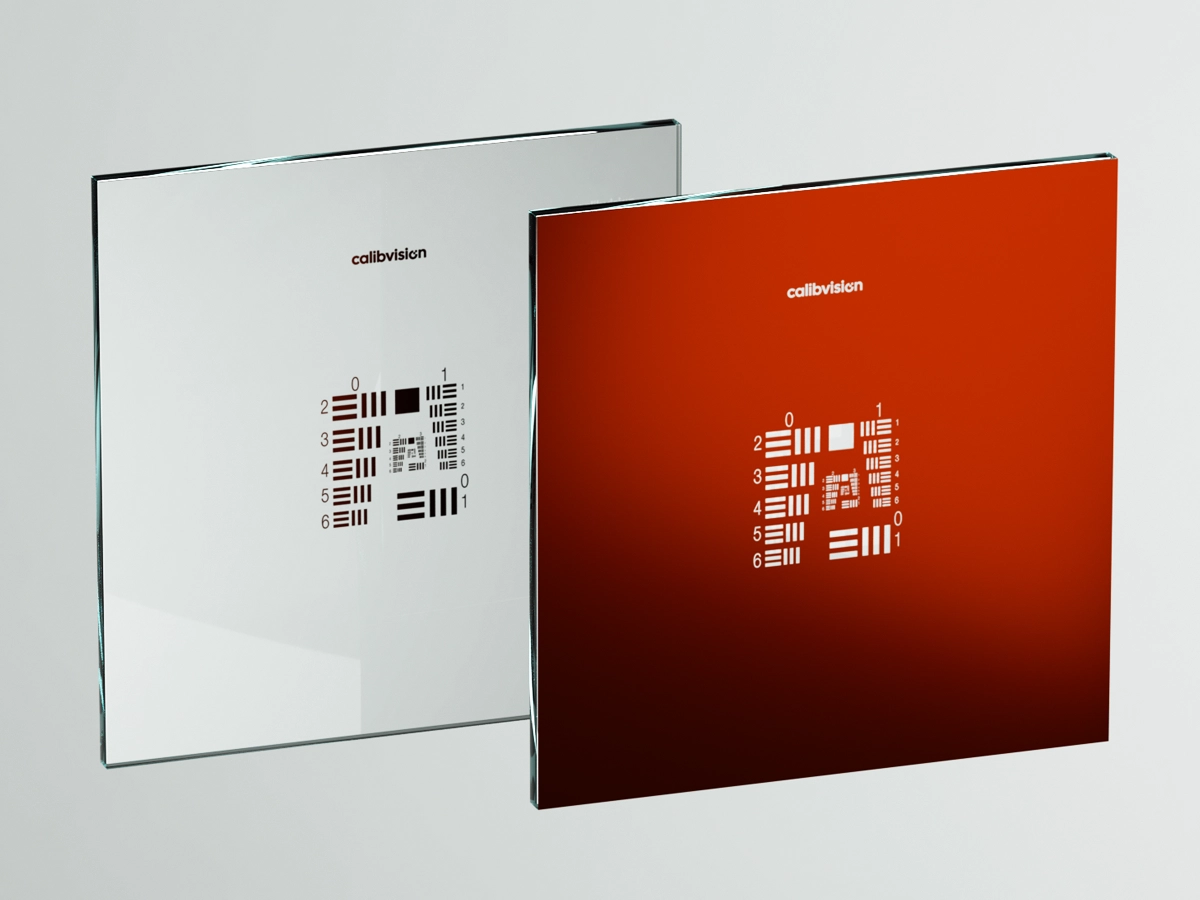
The Anatomy of a USAF 1951 Chart

Every USAF 1951 chart shares the same fundamental structure.

The Three-Bar Pattern

Each element on the chart is a triplet of three parallel bars (plus a corresponding triplet rotated 90°). The bars have equal width and equal spacing — the dark bar width equals the light gap width. This is called a Ronchi ruling in optical terminology.

Why three bars? Because resolving just two bars can sometimes be confused with detecting a single edge. Three bars with equal spacing forces the imaging system to actually resolve the full periodic pattern, not just an edge transition.

Groups and Elements

The chart is organized in a 2D matrix:

• Groups range from −2 to 9 (12 columns total)
• Elements range from 1 to 6 (6 rows)

Each (Group, Element) coordinate gives one specific resolution value. The smaller the group/element numbers, the larger the bars; the larger the numbers, the smaller the bars.

A few reference points:

• Group −2 Element 1: bars 2 mm wide each (0.25 lp/mm) — visible from across the room
• Group 0 Element 1: bars 500 μm wide (1 lp/mm) — clearly visible by eye
• Group 5 Element 1: bars 15.6 μm wide (32 lp/mm) — requires magnification
• Group 9 Element 6: bars 0.55 μm wide (912.30 lp/mm) — only resolvable with a high-NA microscope

The Spatial Layout

The MIL-STD-150A standard arranges 6 groups on a single chart in a compact spiral pattern across 3 nested layers. Odd-numbered groups place Elements 1–6 contiguously from the upper-right corner; even-numbered groups place Element 1 at the lower-right corner with Elements 2–6 on the left side. Look for the printed group/element numbers next to each pattern — they tell you which one you’re looking at.

The Resolution Formula

Resolution (lp/mm) = 2^(Group + (Element − 1) / 6)

With this single formula, you can compute the resolution of any element on the chart in seconds.

Worked Examples

• Group 4 Element 3: 2^(4 + 2/6) = 2^4.333 = 20.16 lp/mm
• Group 7 Element 2: 2^(7 + 1/6) = 2^7.167 = 143.7 lp/mm
• Group 9 Element 6: 2^(9 + 5/6) = 2^9.833 = 912.30 lp/mm

Converting Resolution to Line Width

Line Width (μm) = 1000 / (2 × Resolution in lp/mm)

The factor of 2 appears because one line pair consists of one dark bar plus one light gap (two bar widths total).

Calculating the Theoretical Maximum (Diffraction Limit)

Before testing any optical system, it helps to know what’s theoretically possible. The diffraction limit sets a physical ceiling on resolution that no lens can exceed.

The Two Key Formulas

For most optical engineering work, two criteria define the diffraction limit:

Rayleigh Criterion (the most commonly cited):

Resolution (μm) = 0.61 × λ / NA

Abbe Criterion (slightly more optimistic, often used by microscopists):

Resolution (μm) = 0.5 × λ / NA

Where:

• λ = wavelength of light (usually 0.55 μm for visible green)
• NA = numerical aperture of the objective or lens

The result is the minimum distance between two resolvable points. Converting to line pairs:

Theoretical max (lp/mm) = 1000 / (2 × diffraction resolution in μm)

Quick Reference: NA → USAF Element

This table shows what USAF element your system should theoretically be able to resolve, given its numerical aperture (at λ = 550 nm, Rayleigh criterion):

NA	Diffraction resolution	Max lp/mm	Closest USAF Element
0.1	3.36 μm	149 lp/mm	Group 7 Element 2 (143.7)
0.2	1.68 μm	298 lp/mm	Group 8 Element 2 (287.4)
0.3	1.12 μm	447 lp/mm	Group 8 Element 5 (406.4)
0.4	0.84 μm	596 lp/mm	Group 9 Element 2 (574.7)
0.5	0.67 μm	746 lp/mm	Group 9 Element 4 (724.1)
0.65	0.52 μm	962 lp/mm	Group 9 Element 6 (912.30, chart limit)
0.8	0.42 μm	1,190 lp/mm	Exceeds chart
1	0.34 μm	1,471 lp/mm	Exceeds chart
1.40 (oil)	0.24 μm	2,083 lp/mm	Exceeds chart

Important: For objectives with NA ≥ 0.80, you’ll exceed the USAF 1951 chart’s 912.30 lp/mm ceiling. At these resolutions you’ve reached the chart’s physical limit, not the objective’s. Use a chart with smaller features (custom 2400 lp/mm targets) or switch to MTF-based methods.

Worked Example: 40× Microscope Objective (NA 0.65)

You have a 40× microscope objective with NA = 0.65. Compute the expected USAF reading:

1. Rayleigh resolution: 0.61 × 0.55 / 0.65 = 0.52 μm
2. In line pairs: 1000 / (2 × 0.52) = 961 lp/mm
3. Closest USAF element: Group 9 Element 6 (912.30 lp/mm)

So your 40× / NA 0.65 objective should resolve all the way to the chart’s maximum element. If it can’t — say, it only resolves Group 9 Element 1 (512 lp/mm) — the objective is underperforming and may need alignment, cleaning, or replacement.

Reverse: USAF Element → Inferred NA

Sometimes you measure first and want to back-calculate the system’s effective NA. For example, if your camera lens resolves to Group 7 Element 2 (143.7 lp/mm) at green light:

• Line width at the resolution limit: 1000 / (2 × 143.7) = 3.48 μm
• Required NA: 0.61 × 0.55 / 3.48 = 0.097

So the lens behaves as if it has NA ≈ 0.10 — useful for comparing to specifications or competing optics.

Detailed Test Bench Setup

Real-world USAF reading requires a properly built test bench. Most “the chart doesn’t work” problems trace back to setup errors rather than the chart itself.

Hardware Checklist

For a basic transmission/brightfield setup, you need:

1. The chart itself — choose size by your sensor/objective (more on this in product selection)
2. A chart holder — magnetic mount, microscope slide holder, or precision optical mount with ±1 mm positioning
3. A backlit lightbox — D65 illuminant, ≥98% spatial uniformity, dimmer control for camera exposure flexibility
4. A camera or microscope — with manual focus, ISO/exposure control, RAW output
5. An optical bench or stable surface — anti-vibration table preferred for high-resolution work
6. A working-distance gauge or ruler — for repeatable positioning

For reflection mode (most non-transmission setups), replace the lightbox with two diffuse 45° softboxes mounted equidistant from the chart.

Working Distance Calculation

Many beginners forget this: the chart size you need depends on the working distance and the field of view (FOV).

For a camera lens with focal length f and sensor diagonal d_sensor, the chart should fill at least 60–80% of FOV at your working distance D:

Chart diagonal ≥ 0.7 × (d_sensor × D / f)

Example: A 50 mm lens on a full-frame sensor (43 mm diagonal) at 1 m working distance needs a chart with diagonal ≥ 0.7 × (43 × 1000 / 50) = 602 mm. The 1″ (25×25 mm) chart would only fill 4% of the frame — much too small. Use a 3″ (76×76 mm) or larger custom chart, or move closer.

For microscopes, the chart should fill the entire field number (FN) of the eyepiece converted to specimen-side units: chart size ≈ FN / magnification. A 40× objective with FN 22 mm needs chart features at the specimen plane of about 22/40 = 0.55 mm field of view — meaning a 1″ chart provides far more than enough area; you’ll only use a small central portion.

Lighting Setup (Where 80% of Errors Come From)

For transmission/film charts:

• Use a D65 LED lightbox with CRI ≥ 95 and uniformity ≥ 98% across the chart area
• Avoid fluorescent or incandescent sources — their spectra cause color and contrast issues
• Diffuse the source through ground glass or opal acrylic to eliminate hotspots
• Dim to control camera exposure — never use the camera’s ISO or sharpening to compensate

For reflection/paper-style or ceramic charts:

• Two softboxes at 45° from both left and right of the chart
• Equal distance and equal intensity (verify with a light meter)
• Baffle stray light falling on the camera lens — flare destroys contrast at high resolutions
• Avoid mixed lighting (LED + window light, etc.) — color casts shift the apparent contrast

Camera/Microscope Settings

Always:

• Native sensor resolution — no in-camera downsampling
• Base ISO (ISO 100 for most DSLRs, lowest available for industrial cameras)
• Sharpening = 0, Noise reduction = 0, Contrast = neutral
• RAW format — JPEG compression destroys the high-frequency content you’re trying to measure
• Manual focus — autofocus often locks on the wrong region for resolution charts
• Mirror lock-up (for DSLRs) or electronic shutter (industrial cameras) to eliminate vibration
• Self-timer or remote shutter — finger-press vibration adds blur

Never:

• Trust JPEG output as your reference
• Use a high ISO to “see better”
• Apply in-camera or post-processing sharpening before measurement
• Test handheld

Eliminating Glare and Flare

The single most underrated factor in high-resolution USAF reading is stray light. Sources include:

• Reflections off the back of transmissive film charts → use a black backing or sufficient distance
• Light bouncing from the bench surface → cover with matte black cloth
• Light reaching the lens directly (not via the chart) → install a lens hood and side baffles
• Camera body reflections → cover shiny metal with matte tape during the test

A 1% veiling glare reduces edge contrast by enough to drop your readable element by 1–2 numbers. Take it seriously.

How to Identify the Smallest Resolvable Element

Reading a USAF 1951 chart from a captured image is a visual process.

Step 1 — Set up the imaging system

Mount the chart flat, perpendicular to the optical axis. Illuminate evenly per the setup guide above.

Step 2 — Capture in optimal conditions

Use native resolution and base ISO with sharpening disabled. RAW format preferred. Focus precisely on the central (highest-resolution) region using live view or fine-stage adjustment.

Step 3 — Examine at 100% pixel size

Start at the smallest group on the chart and work outward toward lower groups. For each element, ask: Can I clearly count three distinct dark bars, separated by two distinct light gaps?

Step 4 — Apply the resolution criteria

An element is considered resolved when:

1. All three dark bars are visually distinguishable as separate bars
2. The two light gaps are clearly visible
3. The triplet does not appear as a blurred gray region
4. Contrast modulation is at least 10% (the practical visual threshold)

Step 5 — Record the result

The smallest fully resolved element defines your limiting resolution.

Reading at the System Limit — Distinguishing Real Resolution from Aliasing

Near the system’s resolution limit, your eyes can be deceived. Here’s how to tell genuine resolution from artifacts.

The 10% Contrast Threshold

The Rayleigh-resolved criterion (which the visual threshold approximates) is 10% contrast modulation between bar and gap. Below 10%, the bars look like “ghosts” — visible but degraded. At about 5% modulation, most observers stop calling them resolved.

Practical test: at the smallest still-resolved element, measure the gray level of the darkest and lightest pixels. If they’re within ±5% of each other, you’ve over-claimed resolution by 1–2 elements.

Aliasing — The Trap

When the pattern frequency approaches your sensor’s Nyquist frequency (half the pixel rate), aliasing kicks in. You may see:

• Phantom patterns at the wrong spacing (often perpendicular to the bars)
• Color fringing on monochrome targets (caused by Bayer color filter aliasing)
• Contrast reversal — bars appear bright where they should be dark and vice versa
• Beat patterns that look like resolved bars but with the wrong count

A USAF triplet that shows 4 or 2 bars instead of 3, or where the bars curve, or where adjacent vertical/horizontal triplets disagree — these are aliasing artifacts, not true resolution.

Sub-Pixel Sampling

If your camera produces fewer than 2 pixels per bar at the test element, you’re undersampling. The image may look like “something is there” but the measurement is unreliable. Sanity check: at the smallest claimed-resolved element, count the pixels per bar. You need at least 2; ideally 4 or more.

Orientation Effects

USAF elements come in both horizontal and vertical orientations specifically so you can check orientation-dependent artifacts. If you can resolve the vertical triplet but not the horizontal at the same group/element, your system has horizontal-axis astigmatism or anisotropic sampling (common in many sensors with non-square pixels or directional sharpening).

The “official” limiting resolution is the worst case across both orientations — be conservative.

USAF 1951 Reference Tables

Resolution in Line Pairs per Millimeter (lp/mm)

Element \ Group	−2	−1	0	1	2	3	4	5	6	7	8	9
1	0.25	0.5	1	2	4	8	16	32	64	128	256	512
2	0.281	0.561	1.12	2.24	4.49	8.98	17.96	35.9	71.8	143.7	287.4	574.7
3	0.315	0.63	1.26	2.52	5.04	10.08	20.16	40.3	80.6	161.3	322.5	645.1
4	0.354	0.707	1.41	2.83	5.66	11.31	22.63	45.3	90.5	181	362	724.1
5	0.397	0.794	1.59	3.17	6.35	12.7	25.4	50.8	101.6	203.2	406.4	812.7
6	0.445	0.891	1.78	3.56	7.13	14.25	28.51	57	114	228.1	456.1	912.3

Line Width in Micrometers (μm)

Element \ Group	−2	−1	0	1	2	3	4	5	6	7	8	9
1	2000	1000	500	250	125	62.5	31.25	15.63	7.81	3.91	1.95	0.98
2	1781.8	890.9	445.45	222.72	111.36	55.68	27.84	13.92	6.96	3.48	1.74	0.87
3	1587.4	793.7	396.85	198.43	99.21	49.61	24.8	12.4	6.2	3.1	1.55	0.78
4	1414.21	707.11	353.55	176.78	88.39	44.19	22.1	11.05	5.52	2.76	1.38	0.69
5	1259.92	629.96	314.98	157.49	78.75	39.37	19.69	9.84	4.92	2.46	1.23	0.62
6	1122.46	561.23	280.62	140.31	70.15	35.08	17.54	8.77	4.38	2.19	1.1	0.55

Practical Use Cases

Use Case 1: Microscope Objective Validation — Full Acceptance Protocol

This is the most common professional use of USAF 1951 charts. Here’s the full protocol microscopy labs use to qualify a new or repaired objective.

Setup:

1. Mount a 1″ chart (CV-USAF-1QG-P-(0-9, 6)-BLC recommended) on the microscope’s standard slide holder
2. Place a drop of immersion oil between the objective and chart only if using oil-immersion objectives; otherwise dry
3. Use Köhler illumination with the condenser NA matched to the objective NA (or slightly higher)
4. Centered, neutral filter eyepieces; remove any reticles or polarizers

Test procedure:

1. Focus on a low-resolution element (e.g., Group 5 Element 1) using coarse focus first, then fine focus
2. Translate the stage to bring the highest-resolution group into view
3. Refocus at the high-resolution group (the focus position shifts slightly between groups due to chart thickness)
4. Identify the smallest element where all three bars remain distinct in both horizontal and vertical orientations
5. Repeat the read at three locations: chart center, mid-field, and edge of field
6. Compare to theoretical: Use the NA → lp/mm table above to predict expected performance

Acceptance criteria (typical for production microscopes):

• Center: within 1 element of theoretical (e.g., 40× NA 0.65 should read at minimum Group 9 Element 5 = 812 lp/mm)
• Mid-field: within 2 elements of center
• Edge: within 3 elements of center

If any reading is more than 3 elements below theoretical, the objective fails QC. Common causes: contaminated lens surfaces, mechanical misalignment, or aging coatings.

Use Case 2: Camera Lens Through-Focus MTF (Detailed Procedure)

For lens manufacturers and reviewers, characterizing how MTF varies through focus is essential.

Setup:

1. Mount the lens on a high-precision camera body (ideally a calibrated test bench camera, not a consumer DSLR)
2. Place a 2″ or 3″ USAF chart at a working distance equal to at least 25× the focal length to ensure infinity-like behavior (e.g., 50 mm lens needs ≥1.25 m working distance)
3. Use a D65 backlit lightbox behind the transmissive chart
4. Set the lens at the aperture of interest (typically f/2.8, f/4, f/5.6, f/8 for comparison)

Test procedure:

1. Establish best focus visually using live view at maximum magnification
2. Capture an image and read the limiting USAF element
3. Move the lens focus by a controlled amount (e.g., 50 μm in object space, calculated from the depth of field formula)
4. Capture another image, read the limiting element
5. Repeat for ±0.5 mm range in 0.1 mm steps
6. Plot limiting lp/mm vs focus position

The resulting curve shows:

• Peak position: actual best focus (may not be where the lens scale indicates)
• Peak width: depth of field at your aperture
• Peak height: maximum performance
• Asymmetry: indicates spherical aberration or curvature of field

Pass criteria for a quality 50 mm prime at f/5.6:

• Peak limiting resolution ≥ Group 8 Element 3 (322 lp/mm) at center
• Peak width (±50 lp/mm) ≥ 150 μm

Use Case 3: Machine Vision QC Setup (Real Production Workflow)

Industrial machine vision integrators use USAF 1951 to qualify both the camera and the entire imaging pipeline.

Application requirements example:

• Defect detection: minimum 50 μm feature in the target
• Camera: 2.5 μm pixel pitch, 12 MP (4000 × 3000)
• Lens: industrial macro, 25 mm focal length
• Working distance: 300 mm

Required resolution calculation:

• Field of view at 300 mm distance: 4000 × 2.5 / 25 = 400 mm wide × 300 mm tall
• Pixel size at the target: 400 / 4000 = 100 μm per pixel at the target plane
• To detect 50 μm features, need at least 2 pixels per feature → system must resolve 100 μm features cleanly
• 100 μm = 5 lp/mm at the target plane

Setup procedure:

1. Place a 3″ CV-USAF-3SG-P-(-2-9, 1)-BRC chart at the camera’s working distance (300 mm)
2. Capture under production lighting conditions (don’t add ideal lighting if production doesn’t have it)
3. Find the smallest resolved element in the captured image
4. Convert to “lp/mm at the target”: measured chart lp/mm × (chart size / image width)

Acceptance:

• Required: 5 lp/mm at target → should resolve at least Group 3 Element 1 (8 lp/mm) on the chart with margin
• If the system only resolves Group 2 Element 3 (5 lp/mm) — exactly at the requirement — there’s no margin for production drift. Reject or rebuild.

Use Case 4: Smartphone / Mobile Camera Module Testing

Mobile module factories use USAF 1951 charts for both R&D characterization and incoming sensor QC.

Setup:

• 1″ CV-USAF-1SG-P-(0-9, 1)-BRC (Value Line, sufficient for typical 1.4 μm pixel sensors)
• Custom holder positioning the chart at typical phone-to-subject distances (300-800 mm)
• D65 LED panel for transmission

Production QC threshold:

• 12 MP / 1.4 μm pixel sensor with 4 mm lens at 500 mm distance:
  • System spatial sampling: 1.4 μm × 500 / 4 = 175 μm per pixel at chart
  • Sampling lp/mm at chart: 1000 / (2 × 175) = ~2.85 lp/mm
  • To clearly resolve, need 2× margin → 5.7 lp/mm
  • Closest USAF element: Group 3 Element 1 (8 lp/mm) → minimum acceptance criterion

Modules failing this minimum are rejected at incoming QC.

Common Mistakes When Reading USAF Charts

Mistake 1 — Confusing “lines per mm” with “line pairs per mm”

1 lp/mm = 2 l/mm. USAF 1951 by convention uses lp/mm. Don’t accidentally double or halve numbers across sources.

Mistake 2 — Reading the wrong element due to the spiral layout

Look for the printed numbers next to each group. Don’t assume left-to-right scan.

Mistake 3 — Calling an element resolved when there’s aliasing

See the dedicated “Reading at the System Limit” section above.

Mistake 4 — Ignoring chart manufacturing tolerances

Self-printed USAF charts on consumer printers typically have ±100–500 μm line accuracy. At Group 5 and above (bars under 15 μm), printing tolerances dominate. Professional charts at ±20 nm line tolerance — like the Premium variants in CalibVision’s USAF 1951 line — are required for accurate measurement above Group 5.

Mistake 5 — Reading from a lighting-compromised image

Always use D65, eliminate stray light, verify dark patches show full black.

Mistake 6 — Not checking both orientations

The “official” limiting resolution is the worst case across horizontal and vertical orientations. Many systems have anisotropic sampling or directional aberrations.

Mistake 7 — Trusting JPEG over RAW

JPEG compression applies sharpening that artificially boosts apparent resolution at coarse scales but destroys it at fine scales. Always capture in RAW.

What “Limiting Resolution” Really Tells You

USAF 1951 gives you one number — the finest pattern you can resolve. This is useful, but limited.

What it does tell you

• Whether your system meets a binary pass/fail criterion
• A single performance index for production QC
• An estimate of best-case sharpness for marketing/specs
• Whether two systems differ by enough to matter (i.e., 1+ element difference)

What it doesn’t tell you

• How contrast varies with spatial frequency (the MTF curve)
• Where the rolloff begins (the “knee” of the MTF curve)
• Whether the system has subtle problems at intermediate frequencies (e.g., a dip at 50% Nyquist from sharpening artifacts)
• Acceptance for tasks like text legibility, which depend on contrast at specific frequencies

When USAF reading is enough

• Optical bench setup and alignment
• Microscope objective acceptance testing
• Lens manufacturing QC (sampling)
• Educational and reference work
• Quick comparisons

When you need full MTF analysis

• Lens design optimization
• Camera ISP tuning
• Comparative benchmarking of competing optics
• Tasks requiring a specific contrast at a specific frequency

For full MTF analysis, modern practice uses slanted-edge targets and the Spatial Frequency Response (SFR) method defined in ISO 12233. Software like Imatest computes the full MTF curve from a slanted edge in seconds.

If your work routinely requires MTF curves, consider adding an ISO 12233 test chart or eSFR ISO chart — though for visual limiting resolution of optical hardware, USAF remains the standard.

FAQs

Quick Reference Cheat Sheet

Formula: lp/mm = 2^(Group + (Element − 1) / 6) Line width (μm): 1000 / (2 × lp/mm) Diffraction limit (μm): 0.61 × λ / NA (Rayleigh)

Common values:

Group/Element	lp/mm	Line width	Inferred NA (at 550 nm)
0 / 1	1	500 μm	0.00067
1-Mar	8	62.5 μm	0.0054
1-May	32	15.6 μm	0.022
1-Jul	128	3.91 μm	0.086
1-Sep	512	0.98 μm	0.343
6-Sep	912.3	0.55 μm	0.611

Conclusion

Reading a USAF 1951 chart starts with one formula — lp/mm = 2^(Group + (Element − 1) / 6) — but the difference between an amateur measurement and a professional one comes from understanding the diffraction limit, building a proper test bench, distinguishing real resolution from aliasing, and applying the right acceptance criteria for your industry.

For most optical engineers, microscopists, and machine vision integrators, the procedure above is everything you’ll need for the next decade of work. Bookmark this page, print the cheat sheet, and reach for the formula whenever you need to convert between Group/Element and lp/mm.

Ready to upgrade your test bench?

CalibVision offers 12 standard USAF 1951 SKUs covering both precision tiers, three sizes, both polarities, and resolution coverage from 0.25 to 912.30 lp/mm — all compliant with MIL-STD-150A and shipped with optional NIM-traceable third-party metrology calibration.

Tier	Best for	Resolution	SKU example
Value (Soda Lime Glass + Brown Chrome, ±50 nm)	Production QC, machine vision, education	up to 512 lp/mm	CV-USAF-2SG-P-(0-9, 1)-BRC
Premium (Quartz Glass + Blue Chrome, ±20 nm)	High-power microscopy, semiconductor, R&D	up to 912.30 lp/mm	CV-USAF-2QG-P-(0-9, 6)-BLC